Bias and Variance in Statistics and Machine Learning - Part 2

Bias and Variance in Machine Learning

Attachments

article code.txt (622 B)

In part one of this article, I went through the concepts of bias, variance, and mean square error in a statistical model. In this part of the article, I will explore these terms for a machine learning algorithm. We will see that, while they share similarities in both fields, there are significant deviations.

I will also touch on the idea of a tradeoff between bias and variance in older machine learning algorithms. Interestingly, this tradeoff need not exist for more modern algorithms such as neural networks and random forests.

The Machine Learning Setting

I am using the approach and notation from this excellent set of lecture notes. I will also continue to use the same notation from part one of this article, so as to make it easier to draw parallels between the two contexts.

Suppose we have a set of data $ D_n = \{ (x_1,y_1),...,(x_n,y_n) \} $ of size $ n, $ where each point $ (x_i,y_i) $ is drawn independently from a distribution $ P $ . Just like for part one, to reduce the clutter, I am suppressing the $ n $ in $ D_n, $ and writing it as just $ D. $

Let us call the feature vector $ x_i $ , and $ y_i $ the corresponding label. Now, let $ h_D $ be a model generated by an algorithm when using input data $ D. $ In the lecture notes, $ h_D $ stands for the “Hypothesis calculated from Data”. A linear regression line could be an example of one such model $ h_D. $

$$ \hat{y}_i = \alpha + \beta x_i. $$

The coefficients $ \alpha $ and $ \beta $ are estimated from the data. And $ \hat{y}_i $ is the model’s prediction of $ y_i $ given the input $ x_i. $

Expected Label

This is where we start diverging from thve statistics setting.

In the statistics context, we were trying to estimate a fix parameter of the distribution $ P. $ Here, for the machine learning context, we are given a fixed feature vector $ x $ and we want to predict the corresponding label $ y. $

An added complication here is that the distribution $ P $ might allow different labels to be generated with the same $ x. $ We define the expected label given $ x $ as

$$ \overline{y}(x) = \int_y y \, P(y|x) \, dy. $$

The figure below shows a visualization of an illustration of the concepts we have covered so far, generated using mock data. The python code for this figure can be found in the article code.txt attachment at the top of this article.

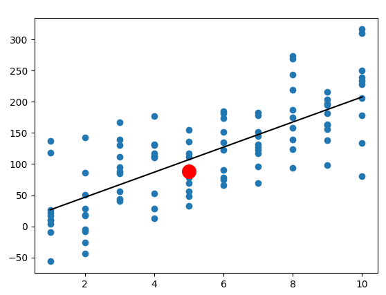
The blue dots represents our dataset $ D. $ The black line is a linear regression line, which is an example of model $ h_D $ that is estimated from the data. For input $ x = 5, $ there is a range of possible labels $ y. $ The rough position of the expected label $ \overline{y}(x) $ for this input is given by the red circle. Note that this setup is also consistent with the case where each feature vector $ x $ correspond to exactly one label ( y ).

Training and Test Dataset, Expected Classifier

Another difference from statistics is that we are often working with two different sets of data. The training dataset $ D $ is first used to build the algorithm $ h_D. $ Then, we randomly draw values $ (x,y) $ from distribution $ P $ to test the efficacy of our model. The latter values form the test dataset.

This separation between two sets of data affects how we take expectations. For example, given a fixed training set $ D $ , we might look at the expected prediction of $ h_D $ on the training set

$$ \mathbb{E}_{(x,y)}[h_D(x)]. $$

We can also take expectations over the training set $ D. $ For example, given a fixed input value $ x $ , we can look at the output of the expected classifier,

$$ \overline{h}(x) = \mathbb{E}_{D}[h_D(x)] = \int_D h_D(x) \, P(D) \, dD. $$

The Mean Square Error

Unlike for the statistics setting, it is easier for me to first decompose the mean square error (MSE) before defining bias and variance. In this case, the mean square error, also known as the expected test error, is

$$ \mathbb{E}_{(x,y),D}[(h_D(x) - y)^2]. $$

Every time we randomly draw a new training dataset $ D, $ we might get a different model $ h_D. $ Then, in order to calculate the square difference between the predictions of the model and the true labels, we randomly draw values $ (x,y) $ from distribution $ P $ for the test dataset. Hence, the expectation is take over all possible training sets $ D, $ and all possible test values $ (x,y) $ .

Important note: there is no unanimous agreement that the expected test error should be defined this way. This is just one common approach.

Also note that we would not be able to perform the same bias-variance decomposition in this article if we defined the test error with a 0-1 loss function instead of the squared deviation. See this paper for an example of that.

Decompositing the Mean Square Error

Like before, we can decompose the MSE into two terms by using the “adding zero” trick to both add and subtract a $ \overline{h}_D(x) $ term into the expectation, and then expanding the square

$$ \begin{align} \mathbb{E}_{(x,y),D}[(h_D(x) - y)^2] &= \mathbb{E}[(h_D - \overline{h} + \overline{h} - y)^2] \\[0.5em] &= \mathbb{E}[(h_D - \overline{h})^2] + \mathbb{E}[ (\overline{h} - y)^2 ] \\[0.5em] &= \text{Var}(h_D) + \mathbb{E}[ (\overline{h} - y)^2 ]. \end{align} $$

Some terms are omitted to reduce clutter. Please refer to the lecture notes for the full derivation. The variance term $ \mathbb{E}[(h_D - \overline{h})^2] $ can be obtained this way. We can interpret this as the expected square deviations of models $ h_D $ from the average or expected classifier $ \overline{h}. $

But unlike before, the second term is not the bias!

Getting the Bias Term

To get the bias term, we apply the “adding zero” trick once again. But this time, we add and subtract the average label $ \overline{y}(x) $ instead. Notice that both the expected classifier and expected label does not depend on ( D ), and hence the expectation is just take over elements ( (x,y) ) from the test set.

$$ \begin{align} \mathbb{E_{(x,y)}}[\overline{h}(x) - y)^2] &= \mathbb{E}[(\overline{h}(x) - \overline{y}(x) + \overline{y}(x) - y)^2] \\[0.5em] &= \mathbb{E}[(\overline{y}(x) - y)^2] + \mathbb{E}[ (\overline{h}(x) - \overline{y}(x))^2 ]. \\[0.5em] &= \mathbb{E}[(\overline{y}(x) - y)^2] + \text{Bias}(h_D). \\[0.5em] \end{align} $$

Again, the full derivation can be found in the lecture notes. The other term is the noise that comes from variations in the dataset and cannot be reduced.

Putting It All Together

Combining everything from before into one equation, we get the well known additive bias-var decomposition for the expected test error of a machine learning algorithm.

$$ \underset{\text{expected test error}}{\mathbb{E}[(h_D - y)^2] \\[0.5em]} = \underset{\text{bias}}{\mathbb{E}[(\overline{h}_D - \overline{y})^2] \\[0.5em]} + \underset{\text{variance}}{ \mathbb{E}[(h_D - \overline{h}_D)^2] \\[0.5em]} + \underset{\text{noise}}{\mathbb{E}[ (\overline{y} - y)^2 ] \\[0.5em]} $$

As usual, some symbols are omitted to reduce clutter.

Bias-Variance Tradeoff

For older machine learning models like linear regression or decision trees, there is this notion of a tradeoff between a model with high bias versus a model with high variance.

High variance: a complicated classifier that fits the training set very well is likely to vary greatly for different training datasets. This reduces the fitted model’s ability to generalize.
High bias: a simple classifier that only roughly fits the training set is likely to be similar to the expected classifier across different training datasets. But the expected classifer itself will likely produce predicted labels that is far from the expected label given by the input.

However, modern machine learning algorithms such as neural networks and random forests can sometimes achieve a perfect fit on the training set, and yet not suffer from high variance! Below is a great figure from a research paper that does a great job of illustrating this.

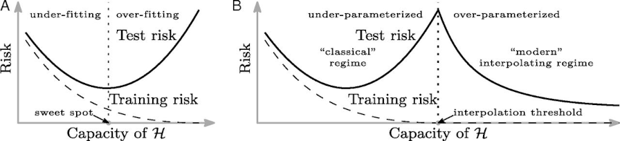
Image source: https://www.pnas.org/content/116/32/15849.

Connection to Statistical Setting

There is one last thing to mention before we finish up. In the previous statistical setting, the bias part of the decomposition refers to the squared bias $ (\mathbb{E}(h_D) - y)^2. $ It is possible to get something similar if we consider the MSE of a single fixed input $ x_0. $ Then, the expectation goes away, and we can get a similar squared bias expression,

$$ (\overline{h}(x_0) - \overline{y}(x_0))^2. $$