Logistic Regression - Part 2

Data Cleaning, Multicollinearity, and Recipe Labels

I briefly went through some of the mathematics behind logistic regression in part 1 of this article. Here, I will use logistic regression to label recipes from www.epicurious.com, as breakfast or not breakfast.

A model like this, when extended to lunch and dinner labels, can be used to suggest labels for new or unlabeled recipes. This should be paired with a mechanism for users to flag inaccurate labels, similar to how Reddit’s automated system that ask users of a community the descriptive labels they generated for that community are accurate.

Let us start by examining the data and discuss the problems that we find with it.

Cleaning the Data

We will be working with this set of data that was generously uploaded to Kaggle and made publicly available here: https://www.kaggle.com/hugodarwood/epirecipes/

The csv file provided has 20052 rows and 680 columns. The rows are the recipes, while the columns are a mix of nutritional information (calories, sodium, fat etc), and binary variables indicating whether an ingredient or a label is present in a recipe.

Missing Data Entries

Many of the recipes are missing nutritional information, seemingly at random as far as I can tell. I chose to simply eliminate these rows. We will see from the results later that this ended up not having much of an impact. I might revisit the topic of missing data and imputation in the future. After this, we are left with 15864 recipes.

Extreme Outliers

Next, we plot the four nutrition columns and see that there are some extreme outliers.

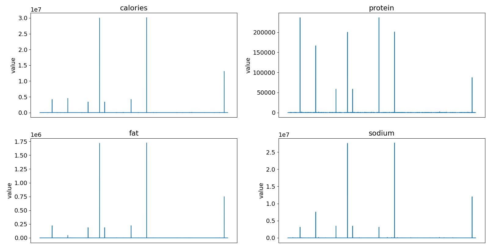
We can plot the number of recipes with nutrition values above various thresholds to get an idea of what the problematic data points look like. We can see from these plots that the problem lies with a handful of recipes having nutritional values in the thousands.

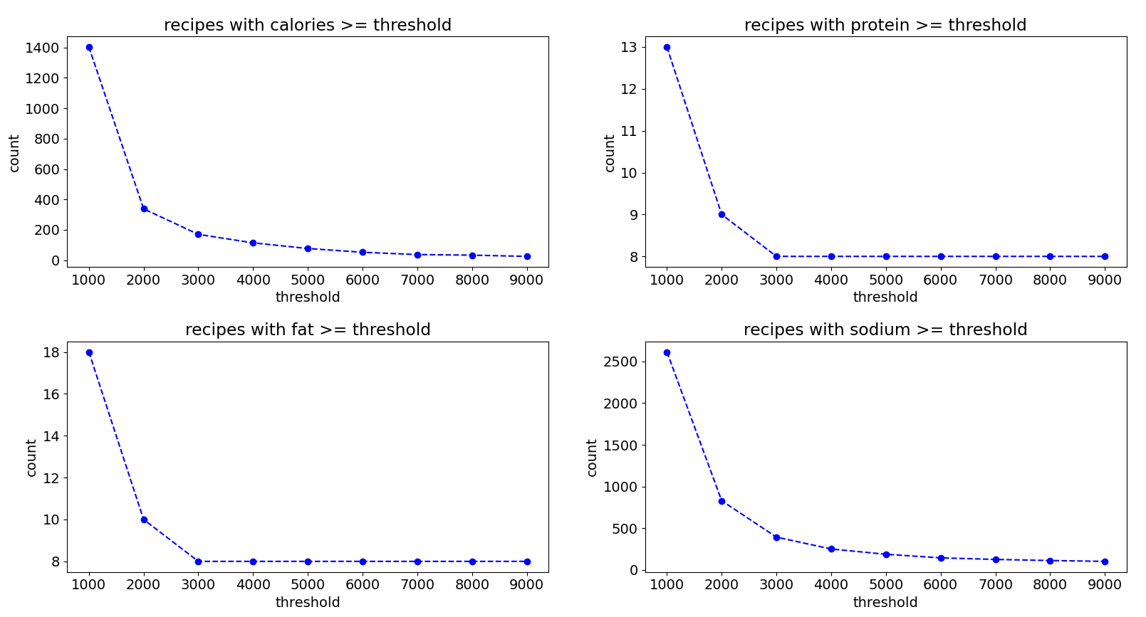
Just like before, these errors appeared to be random, as far as I could tell. So, I used a quick and dirty solution of simply removing all recipes that have calories or sodium values that are equal to or greater than 5000. This ended up also removing recipes with extreme values for protein and fat, leaving only recipes with protein and fat values that are 600 or less. Again, we will see later that not doing more complicated missing value imputation would not have much of an impact.

data = data[data['calories'] < 5000]
data = data[data['sodium'] < 5000]

sum(data['protein'] > 600) # result = 0
sum(data['fat'] > 600) # result = 0

Breakfast, Lunch, Dinner Labels

Lastly, we trim the data down to just recipes that have one and only one breakfast, lunch or dinner label. There could be valid reasons for having more than one label. For example, some dishes can be considered both lunch and dinner. However, for this project, I am just going to focus on recipes with only one label.

label_sum = (data['breakfast'] + data['lunch'] + data['dinner'])
data = data[(label_sum > 0) & (label_sum < 2)]

len(data) # 2460
sum(data['breakfast'] == 1) + sum(data['lunch'] == 1) + sum(data['dinner'] == 1) #2460

After all this cleaning, 130 columns ended up containing nothing but zeroes, and so were dropped. We also drop the “brunch” column since it just repeats information from the breakfast and lunch labels.

The final dataset contains 2460 recipes and 549 columns. The python code for everything we have done up to this point can be found in the data_cleaning.txt file, at the top attachment section of this article.

Multicollinearity

There is one last thing that we need to do, before we can finally run our logistic regression analysis, is to look at the correlations between our independent variables $ \{ x_1,...,x_n \}. $

The $i$-th regression coefficient $ \beta_i $ represents the unit change in the log odds with respect to a unit change in $ x_i, $ while keeping all other variables constant. $ \beta_i $ essentially isolates the effect of $ x_i. $ This is difficult to do when $ x_i $ is highly correlated with another variable $ x_j. $

In that case, both variables will tend to move together. Any change in $ x_i $ will result in a change in $ x_j. $ This makes it hard to isolate the effect of $ x_i $ while keeping all other variables constant. This problem is known as multicollinearity.

There is no official definition of “highly correlated”. For this project, we will just go with an arbitrary threshold of $ 0.85 $ for the pearson correlation coefficient.

# data generated by our cleaning process
temp_data = pd.read_csv('cleaned_data.csv')

C = temp_data.drop(columns = ["breakfast", "lunch", "dinner"])
C = C.corr()
C[C == 1.0] = 0.0 # disregard 1s on diagonals

# see how many variable pairs meet our criteria
(C > 0.85).sum().sum() # result = 6
(C < -0.85).sum().sum() # result = 0

high_corr = C[(C>0.85).sum()==1]
row_names = list(high_corr.index)

# sub-matrix consisting of only > 0.85 correlation
high_corr[row_names]

The pandas package has convenient tools for generating and working with the correlation matrix, which we used to find that none of the variables have correlation, and that six variables have correlation with some other variables. These six variables are shown below.

It makes sense that recipes that are high in fat are also high in calories, and portland is a city in oregon. However, the high correlation between being a drink and being non-alcoholic is interesting, and tells us that most of the beverage recipes in the dataset are non-alcoholic.

Out of each pair of highly correlated variables, I chose to drop the more narrow ones (fat, portland, and non-alcoholic), while keeping the more general ones.

Labeling Breakfast Recipes

We can finally fit the logistic regression model for breakfast labels. The python code for removing highly correlated variables and fitting the model can be found in the breakfast_labels.txt file, at the top attachment section of this article.

Separability

Surprisingly, I was able to get a perfect separation! This would explain why I had some minor problems getting the solver to converge. Iterative solvers have a hard time converging for perfectly separable data because the likelihood has no maximum and can be increased indefinitely.

Upon further inspection of the data, it is easy to see why the data was so easily separated. Out of 15864 recipes, only 493 have breakfast labels. However, there are 542 features, which is more than the number of breakfast labels. This situation is similar to having an overdetermined system in linear algebra. The 542 labels were able to perfectly and completely determine those 493 breakfast labels.

Bias and Generalizability

Lunch and dinner labels appear to be in the same situation and have the same problem. My guess is that these tiny pool of recipes containing only one breakfast/lunch/dinner label were only this way because they were easily identifiable as only breakfast, lunch or dinner. In fact, 12755 out of 15864 recipes are missing labels.

This means that models fitted on this biased sample are unlikely to generalize well to the rest of the dataset. The situation is similar to building a crime prediction model on people who have been arrested before and finding out that the results do not generalize to the rest of the population. People who have been arrested form a biased sample.

Ingredients in Labeled Breakfast Recipes

Given the various issues found with this dataset, I decided to end this project at just briefly looking at breakfast labels. This is too bad since I could have been able to try doing multiclass classification and compare methods such as softmax (multinomial), one vs all, and one vs one. I will also be skipping the usual machine learning process of doing cross validation and examining metrics such as AUC, precision and recall.

Let’s take a look at top 30 and bottom 30 explanatory variables for predicting breakfast labels, in terms of the values of the fitted coefficients.

This is just taking a quick look and not the correct way to determine variable importance in logistic regression models. For example, the absolute value of a coefficients is dependent on the variable unit of measure. However, it looks like they are all binary variables and hence not affected by the unit of measure issue. They are also exactly what we would expect to be in or not in breakfast recipes.

There were a few I thought were mistakes or inaccuracies, but ended up being correct! For example, “hot pepper” turns out to be common among scrambled eggs and egg-based breakfast recipes in the dataset. I also learned that semolina porridge and tofu scramble are breakfast items, and that sake salmon is a Japanese breakfast dish!

Also keep in mind that having a single ingredient in the “top 30” list does not automatically make a recipe breakfast. For example, out of 269 recipes containing “egg”, only 98 of them were lunch or dinner. This is a multivariate model. The final output depends on multiple variables and not just one.

Side Note: p-values are not reported by sklearn’s “linear_model” module, even if regularization is disabled. The statsmodel package is an alternative that does provide p-values.