Logistic Regression - Part 1
Mathematical Theory
Suppose we want to predict a label $ \hat{y}_i $ based on input features $ \{ x_1, \dots, x_n \} $ . Using linear regression, the model that we are fitting to the data is,
Consider the case when the labels are binary. i.e. $ y_i = 0 $ or $ y_i = 1. $ The linear regression model is unlikely to produce $ \hat{y}_i $ values of exactly $ 0 $ or $ 1 $ . In fact, most of the time, values will end up much greater than $ 1 $ or be far below $ 0. $ To get around this problem, we could instead try to fit the logistic regression model,
Where $ \hat{p}_i $ is the model’s estimate of the probability that $ y_i = 1 $ . This estimate is guaranteed to lie between $ 0 $ and $ 1 $ . Plotting the function for values of $ z $ between $ -10 $ and $ 10 $ shows why this is the case.

Model Interpretation
The two terms following $ \hat{p}_i $ above are simply two different ways of writing the logistic function.
A second way of looking at the logistic regression model is that the natural logarithm of the odds $ \frac{ \hat{p}_i }{1 - \hat{p}_i } $ is a linear combination of input $ \{ x_1,...,x_n. \} $ That is,
A third and rather intuitive way of interpreting the model is to note that the function $ f(z) = \frac{1}{1 + e^{-z}} $ is greater than $ \frac{1}{2} $ only when $ z > 0 $ . If our rule is to assign $ \hat{y}_i = 1 $ only when $ \hat{p}_i > \frac{1}{2} $ , then we are looking for a linear separator,
$$ \beta_0 + \beta_1 x_1 + ... + \beta_n x_n > 0. $$These interpretations highlight the fact that logistic regression is a linear model. There are a surprisingly large number of other ways to interpret the logistic regression model. However, as far as I can tell, there is no precise mathematical reason why this model is the “correct” one in any particular situation.
In fact, the logistic function is very similar to the probit function, which is another popular choice for handling binary classification. Sometimes, the choice of model is arbitrary. “All models are wrong, some are useful”.
Deriving and Fitting the Model
The main motivation for the logit model was the desire to apply linear regression methods to probabilities. The following train of thought might approximate what the creators of the model had in mind, and how they arrived at modeling the log odds as a linear combination of input features.
-
We want the fitted probability $ \hat{p}_i $ to be dependent on input $ \{ x_1,...,x_n \} $ , in a way that is somehow linear.
-
We want $ \hat{p}_i $ to be within the interval $ (0, 1) $ .
-
We want to incorporate diminishing returns, so that it takes a bigger change to make a large $ \hat{p}_i $ larger, or a small $ \hat{p}_i $ smaller.
This set of lecture notes contains a discussion about this line of reasoning, and goes through the derivation of logistic regression in much greater mathematical details.
When it comes to fitting the model, the “best” set of parameters $ \{ \beta_0, \beta_1, ..., \beta_n \} $ is defined to be the one that maximizes the probability of generating our data. This is known as maximum likelihood estimation. However, there is no way to solve for these parameters exactly. Numerical methods such as Newton’s method would have to be used.
Comparison with Linear Regression
Why don’t we just use linear regression? Well, I gave a couple of reasons in the previous section.
That being said, we could try to use linear regression for binary classification with a two step process: fit the regression line as usual, pick a threshold, then classify all points with predicted values above this threshold as a $ 1. $ For example, in the figure below, a threshold of $ \hat{y}_i >= 0.50 $ could be used to label $ y_i = 1. $
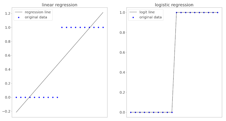
However, since linear regression was not formulated for binary classification, this process could result in corner cases and abnormalities. These figures illustrate yet another possible reason to use logistic regression instead of linear regression: the desire to obtain a closer fit to the data.
With the introduction and mathematical foundations out of the way, we can start working with data in part 2 of this article.